Data Exercise: Analysis of age, gender effects on night time sleep using a synthetic dataset
In this exercise, I chose to work with a dataset that simulates human sleep behavior, focusing on the circadian rhythm, the natural sleep cycle over 24 hours. The dataset includes information from different types of people, organized by age group (like children, adults, elders, and newborns) and gender (female and male), including also sleeping disorder (Regular, or Insomniac).
It records how much people sleep during what was defined by the nigh time hours (from 10 PM to 8 AM), and allows us to explore how age, gender, and whether someone is an insomniac or not affects the number of hours they sleep.
First step was to generate a synthetic dataset.
The code below simulates sleep patterns for different types of people. Each person was randomly assigned a group (“Normal” or “Insomniac”), a gender, and an age, which was then used to classify them into an age type (like “Child”, “Adult”, “Newborn”, or “Elder”).
The 24-hour day was split into 12 time bins, each 2 hours long (e.g., 00–02, 02–04, …, 22–24). For each person, the code calculated how much of their sleep happened in each bin, based on their bedtime and sleep duration.
library(dplyr)
Warning: package 'dplyr' was built under R version 4.4.3
Attaching package: 'dplyr'
The following objects are masked from 'package:stats':

    filter, lag
The following objects are masked from 'package:base':

    intersect, setdiff, setequal, union
library(tidyr)
Warning: package 'tidyr' was built under R version 4.4.3
library(ggplot2)
Warning: package 'ggplot2' was built under R version 4.4.3
set.seed(1)# Define simulation parametersn <-100groups <-c("Regular", "Insomniac")bins <-seq(0, 24, by =2)labels <-paste0(sprintf("%02d", bins), "-", sprintf("%02d", (bins +2) %%24))## AI Disclosure: this part below was created with the assistance of ChatGPT: # Simulate individualssimulate_sleep <-function(group) {# Randomly assign age type age_type <-sample(c("Newborn", "Child", "Adult", "Elder"), 1, prob =c(0.1, 0.1, 0.7, 0.1)) age <-switch(age_type,"Newborn"=round(runif(1, 0.1, 1.5), 2),"Child"=round(runif(1, 3, 12), 1),"Adult"=round(rnorm(1, 35, 10)),"Elder"=round(rnorm(1, 70, 5)))# Set sleep patterns based on Age_type so it can create a correlation. if (age_type =="Newborn") { start <-rnorm(1, 20, 1) dur <-rnorm(1, 10, 1) } elseif (age_type =="Child") { start <-rnorm(1, 21, 0.5) dur <-rnorm(1, 9, 0.7) } elseif (group =="Regular") { start <-rnorm(1, 22.5, 0.5) dur <-rnorm(1, 7.5, 0.5) } elseif (group =="Insomniac") { start <-rnorm(1, 2.0, 1.5) dur <-rnorm(1, 6, 1.5) } gender <-sample(c("Male", "Female"), 1) start <- start %%24 end <- (start + dur) %%24return(data.frame(start, end, duration = dur, group, age, gender, Age_type = age_type))}# Simulate all individualssleep_df <-do.call(rbind, lapply(groups, function(g) {do.call(rbind, replicate(n, simulate_sleep(g), simplify =FALSE))}))# Allocate sleep into time binsallocate_sleep <-function(start, end, duration) { hour_vec <-numeric(length(bins))for (i inseq_along(bins)) { bin_start <- bins[i] bin_end <- (bin_start +2) %%24 in_bin <-function(t) {if (bin_start < bin_end) return(t >= bin_start & t < bin_end)elsereturn(t >= bin_start | t < bin_end) } bin_time <-seq(0, duration, by =0.25) + start bin_time <- bin_time %%24 hour_vec[i] <-mean(in_bin(bin_time), na.rm =TRUE) * duration }return(hour_vec)}# Bin sleep datasleep_binned <- sleep_df %>%rowwise() %>%mutate(sleep_vec =list(allocate_sleep(start, end, duration))) %>%ungroup()# Wide format for averagingsleep_matrix <- sleep_binned %>%select(group, gender, age, Age_type, sleep_vec) %>%unnest_wider(sleep_vec, names_sep ="_") %>%rename_with(~labels, starts_with("sleep_vec"))# Create summary table: average sleep per 2-hour bin by Age_typesleep_summary <- sleep_matrix %>%group_by(Age_type) %>%summarise(across(all_of(labels), mean), .groups ="drop")
    group              gender               age          Age_type
 Length:200         Length:200         Min.   : 0.21   Length:200
 Class :character   Class :character   1st Qu.:20.00   Class :character
 Mode  :character   Mode  :character   Median :33.00   Mode  :character
                                       Mean   :32.52
                                       3rd Qu.:45.00
                                       Max.   :77.00
     00-02            02-04           04-06           06-08
 Min.   :0.0000   Min.   :0.000   Min.   :0.000   Min.   :0.0000
 1st Qu.:0.7435   1st Qu.:1.936   1st Qu.:1.486   1st Qu.:0.0000
 Median :1.9540   Median :1.959   Median :1.944   Median :0.2466
 Mean   :1.4451   Mean   :1.768   Mean   :1.661   Mean   :0.6714
 3rd Qu.:1.9756   3rd Qu.:1.978   3rd Qu.:1.972   3rd Qu.:1.2347
 Max.   :1.9996   Max.   :2.000   Max.   :1.998   Max.   :1.9976
     08-10            10-12             12-14              14-16       16-18
 Min.   :0.0000   Min.   :0.00000   Min.   :0.000000   Min.   :0   Min.   :0
 1st Qu.:0.0000   1st Qu.:0.00000   1st Qu.:0.000000   1st Qu.:0   1st Qu.:0
 Median :0.0000   Median :0.00000   Median :0.000000   Median :0   Median :0
 Mean   :0.2089   Mean   :0.04059   Mean   :0.002489   Mean   :0   Mean   :0
 3rd Qu.:0.0000   3rd Qu.:0.00000   3rd Qu.:0.000000   3rd Qu.:0   3rd Qu.:0
 Max.   :1.9976   Max.   :1.99092   Max.   :0.497730   Max.   :0   Max.   :0
     18-20             20-22            22-00           24-02
 Min.   :0.00000   Min.   :0.0000   Min.   :0.000   Min.   :0.0000
 1st Qu.:0.00000   1st Qu.:0.0000   1st Qu.:0.000   1st Qu.:0.7435
 Median :0.00000   Median :0.0000   Median :1.240   Median :1.9540
 Mean   :0.06315   Mean   :0.3257   Mean   :1.057   Mean   :1.4451
 3rd Qu.:0.00000   3rd Qu.:0.2442   3rd Qu.:1.954   3rd Qu.:1.9756
 Max.   :1.99245   Max.   :1.9976   Max.   :2.000   Max.   :1.9996
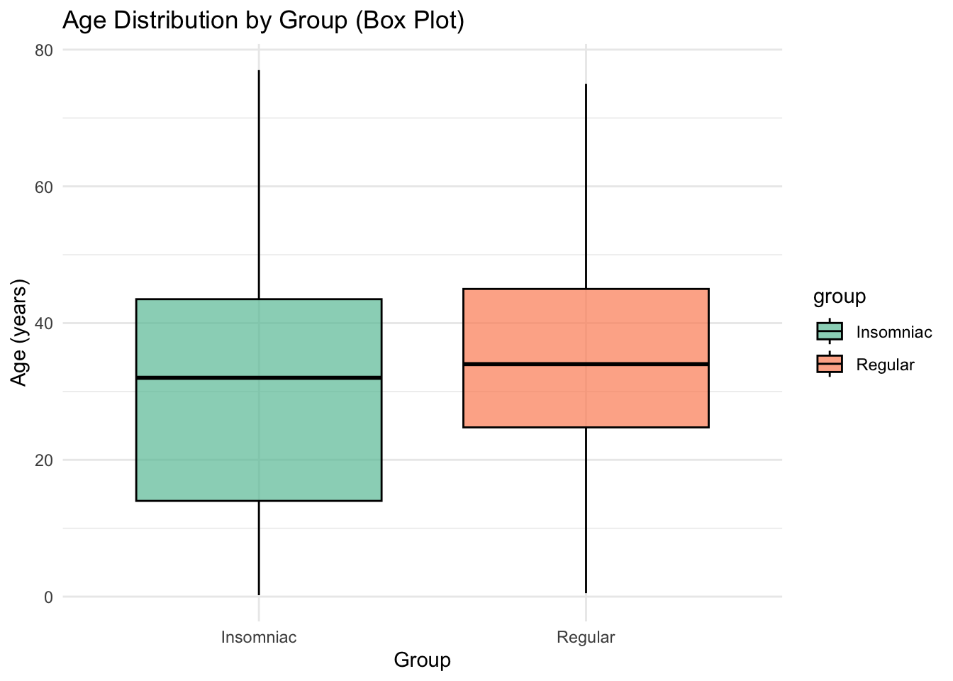
Box Plot showing age of people that has insominia
ggplot(sleep_matrix, aes(x = group, y = age, fill = group)) +geom_boxplot(color ="black", alpha =0.7) +scale_fill_brewer(palette ="Set2") +labs(title ="Age Distribution by Group (Box Plot)",x ="Group", y ="Age (years)") +theme_minimal()
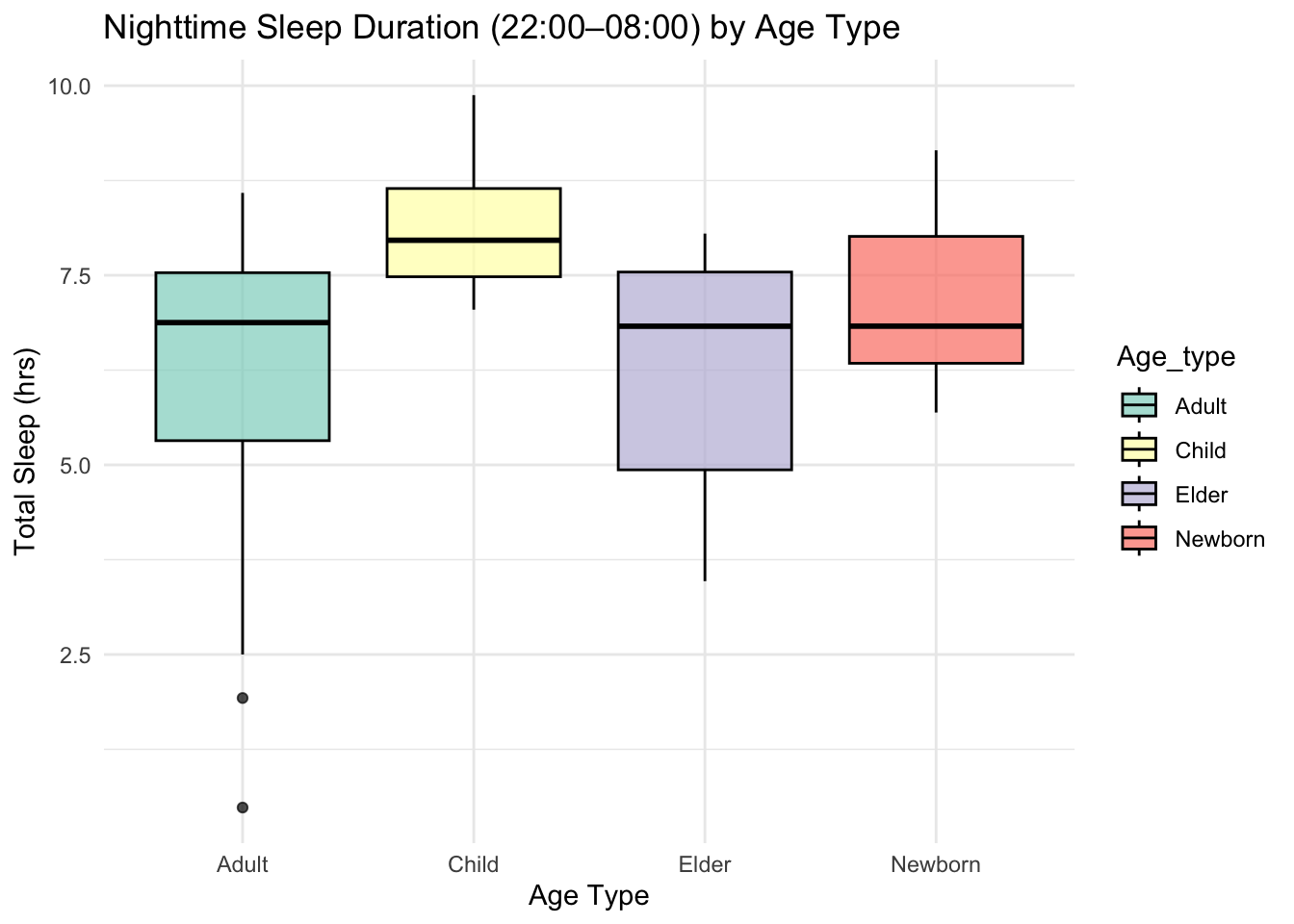
Box Plot of sleep time at night (from 22:00 to 08:00) and age_type (Adult, Child, Elder, Newborn):
# Step 1: Define nighttime binsnight_bins <-c("22-00", "00-02", "02-04", "04-06", "06-08")# Step 2: Calculate total nighttime sleep per personsleep_night <- sleep_matrix %>%mutate(Night_sleep =rowSums(select(., all_of(night_bins)), na.rm =TRUE))# Step 3: Plot boxplot of nighttime sleep by Age_typeggplot(sleep_night, aes(x = Age_type, y = Night_sleep, fill = Age_type)) +geom_boxplot(color ="black", alpha =0.7) +scale_fill_brewer(palette ="Set3") +labs(title ="Nighttime Sleep Duration (22:00–08:00) by Age Type",x ="Age Type", y ="Total Sleep (hrs)") +theme_minimal()
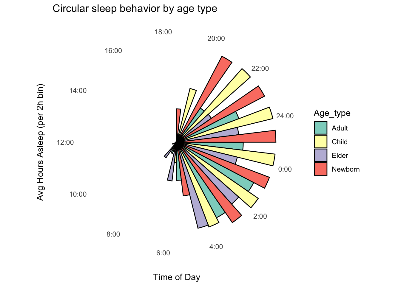
Circular plot of sleep time per category:
# Convert to long format for circular plotsleep_long <- sleep_summary %>%pivot_longer(-Age_type, names_to ="time_bin", values_to ="sleep_amount") %>%mutate(bin_start =as.numeric(substr(time_bin, 1, 2)),bin_label =paste0(bin_start, ":00"),bin_angle =2* pi * bin_start /24 )# Plot circular behavior by Age_typeggplot(sleep_long, aes(x =factor(bin_start), y = sleep_amount, fill = Age_type)) +geom_bar(stat ="identity", position ="dodge", width =1, color ="black") +coord_polar(start = pi/2) +scale_x_discrete(labels =function(x) paste0(x, ":00"),breaks =as.character(bins) ) +labs(title ="Circular sleep behavior by age type",x ="Time of Day", y ="Avg Hours Asleep (per 2h bin)") +scale_fill_brewer(palette ="Set3") +theme_minimal() +theme(axis.text.y =element_blank(),panel.grid =element_blank(),axis.title.y =element_text(margin =margin(r =10)))
Check if the variables predict sleep time:
# Model 1: Predict nighttime sleep using Age_typefit1 <-lm(Night_sleep ~ Age_type, data = sleep_night)summary(fit1)
Call:
lm(formula = Night_sleep ~ Age_type, data = sleep_night)

Residuals:
    Min      1Q  Median      3Q     Max
-5.8659 -0.9613  0.3760  1.1427  2.2386

Coefficients:
                Estimate Std. Error t value Pr(>|t|)
(Intercept)      6.34773    0.11994  52.925  < 2e-16 ***
Age_typeChild    1.77574    0.32898   5.398 1.94e-07 ***
Age_typeElder   -0.07072    0.31634  -0.224    0.823
Age_typeNewborn  0.81264    0.34367   2.365    0.019 *
---
Signif. codes:  0 '***' 0.001 '**' 0.01 '*' 0.05 '.' 0.1 ' ' 1

Residual standard error: 1.404 on 196 degrees of freedom
Multiple R-squared:  0.1456,    Adjusted R-squared:  0.1325
F-statistic: 11.13 on 3 and 196 DF,  p-value: 8.845e-07
lm(formula = Night_sleep ~ Age_type, data = sleep_night)
The model shows that Age_type significantly predicts night time sleep, with Children and Newborns sleeping significantly more than Adults. Elders do not differ significantly from Adults, and the model explains about 14.6% of the variance in sleep duration (R² = 0.1456).
# Model 2: Predict nighttime sleep using genderfit2 <-lm(Night_sleep ~ gender, data = sleep_night)summary(fit2)
Call:
lm(formula = Night_sleep ~ gender, data = sleep_night)

Residuals:
    Min      1Q  Median      3Q     Max
-6.0760 -1.0078  0.4585  1.0249  3.3177

Coefficients:
            Estimate Std. Error t value Pr(>|t|)
(Intercept)   6.6396     0.1434  46.311   <2e-16 ***
genderMale   -0.0818     0.2149  -0.381    0.704
---
Signif. codes:  0 '***' 0.001 '**' 0.01 '*' 0.05 '.' 0.1 ' ' 1

Residual standard error: 1.511 on 198 degrees of freedom
Multiple R-squared:  0.000731,  Adjusted R-squared:  -0.004316
F-statistic: 0.1448 on 1 and 198 DF,  p-value: 0.7039
lm(formula = Night_sleep ~ gender, data = sleep_night)
The model shows that gender does not significantly predict night time sleep duration. Difference that is not statistically significant (p = 0.704).
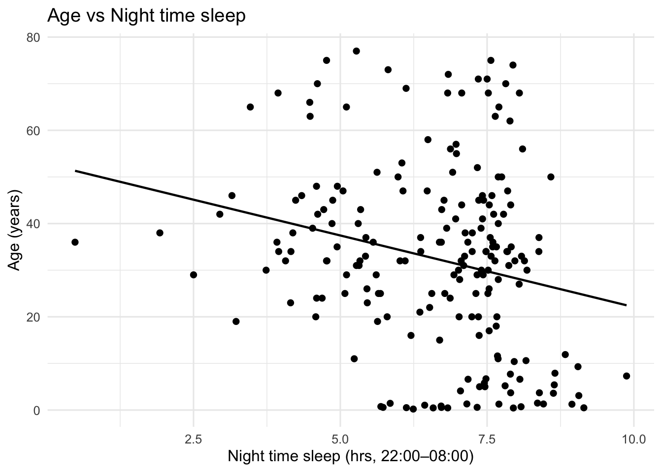
# Model 3: Predict night time sleep using agefit3 <-lm(Night_sleep ~ age, data = sleep_night)summary(fit3)
Call:
lm(formula = Night_sleep ~ age, data = sleep_night)

Residuals:
    Min      1Q  Median      3Q     Max
-6.0604 -1.0861  0.3997  1.0539  2.8303

Coefficients:
             Estimate Std. Error t value Pr(>|t|)
(Intercept)  7.173229   0.199109  36.027  < 2e-16 ***
age         -0.017527   0.005222  -3.356 0.000947 ***
---
Signif. codes:  0 '***' 0.001 '**' 0.01 '*' 0.05 '.' 0.1 ' ' 1

Residual standard error: 1.47 on 198 degrees of freedom
Multiple R-squared:  0.05383,   Adjusted R-squared:  0.04905
F-statistic: 11.26 on 1 and 198 DF,  p-value: 0.0009475
lm(formula = Night_sleep ~ age, data = sleep_night)
Call:
lm(formula = Night_sleep ~ age, data = sleep_night)

Coefficients:
(Intercept)          age
    7.17323     -0.01753
The model indicates that age is a statistically significant predictor of night time sleep, with each additional year of age associated with a decrease of ~0.018 hours (just over 1 minute) in sleep duration (p = 0.00095). However, the effect size is small and the model explains only ~5.4% of the variance in night time sleep (R-squared: 0.05383).
ggplot(sleep_night, aes(x = Night_sleep, y = age)) +geom_point(color ="black", size =1.8) +geom_smooth(method ="lm", color ="black", se =FALSE, linewidth =0.8) +labs(title ="Age vs Night time sleep",x ="Night time sleep (hrs, 22:00–08:00)",y ="Age (years)") +theme_minimal(base_size =12)
`geom_smooth()` using formula = 'y ~ x'
# Model 4: Predict nighttime sleep using group (insomnia status)fit4 <-lm(Night_sleep ~ group, data = sleep_night)summary(fit4)
Call:
lm(formula = Night_sleep ~ group, data = sleep_night)

Residuals:
    Min      1Q  Median      3Q     Max
-5.1988 -0.5934 -0.0280  0.5262  3.4674

Coefficients:
             Estimate Std. Error t value Pr(>|t|)
(Intercept)    5.6806     0.1193   47.61   <2e-16 ***
groupRegular   1.8453     0.1687   10.94   <2e-16 ***
---
Signif. codes:  0 '***' 0.001 '**' 0.01 '*' 0.05 '.' 0.1 ' ' 1

Residual standard error: 1.193 on 198 degrees of freedom
Multiple R-squared:  0.3766,    Adjusted R-squared:  0.3734
F-statistic: 119.6 on 1 and 198 DF,  p-value: < 2.2e-16
lm(formula = Night_sleep ~ group, data = sleep_night)
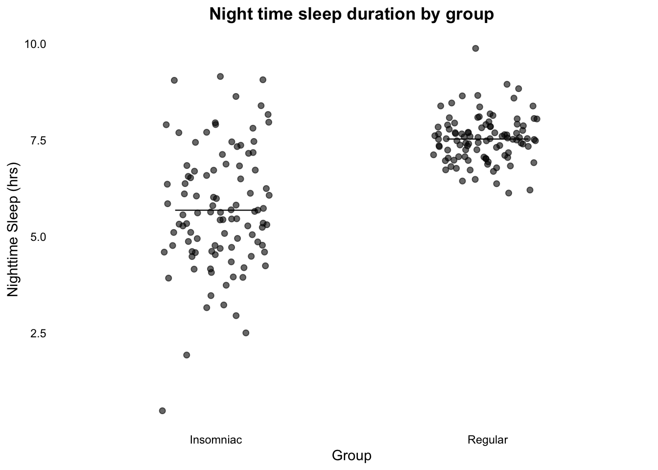
This model shows that group is a strong and highly significant predictor of sleep duration (p < 2e-16). On average, individuals in the Regular (Normal) group sleep 1.85 hours more than those in the Insomniac group.
ggplot(sleep_night, aes(x = group, y = Night_sleep)) +geom_jitter(width =0.2, height =0, color ="black", size =1.8, alpha =0.6) +stat_summary(fun = mean, geom ="crossbar", width =0.3, color ="black", fatten =0.8) +labs(title ="Night time sleep duration by group",x ="Group", y ="Nighttime Sleep (hrs)") +theme_minimal() +theme(panel.grid =element_blank(),axis.text =element_text(color ="black"),axis.title =element_text(color ="black"),plot.title =element_text(hjust =0.5, face ="bold") )
Warning: The `fatten` argument of `geom_crossbar()` is deprecated as of ggplot2 4.0.0.
ℹ Please use the `middle.linewidth` argument instead.