Fitting Exercise

Importing and exploring the data

library(tidyverse)

Warning: package 'ggplot2' was built under R version 4.4.3

Warning: package 'tibble' was built under R version 4.4.3

Warning: package 'tidyr' was built under R version 4.4.3

Warning: package 'readr' was built under R version 4.4.3

Warning: package 'purrr' was built under R version 4.4.3

Warning: package 'dplyr' was built under R version 4.4.3

Warning: package 'lubridate' was built under R version 4.4.3

── Attaching core tidyverse packages ──────────────────────── tidyverse 2.0.0 ──
✔ dplyr     1.2.0     ✔ readr     2.2.0
✔ forcats   1.0.1     ✔ stringr   1.6.0
✔ ggplot2   4.0.2     ✔ tibble    3.3.1
✔ lubridate 1.9.5     ✔ tidyr     1.3.2
✔ purrr     1.2.1     
── Conflicts ────────────────────────────────────────── tidyverse_conflicts() ──
✖ dplyr::filter() masks stats::filter()
✖ dplyr::lag()    masks stats::lag()
ℹ Use the conflicted package (<http://conflicted.r-lib.org/>) to force all conflicts to become errors

library(here)

here() starts at /Users/ayllaermland/Downloads/BIOS8060E/AyllaErmland-portfolio

# Load dataset
data <- read_csv(here("fitting-exercise", "Mavoglurant_A2121_nmpk.csv"))

Rows: 2678 Columns: 17
── Column specification ────────────────────────────────────────────────────────
Delimiter: ","
dbl (17): ID, CMT, EVID, EVI2, MDV, DV, LNDV, AMT, TIME, DOSE, OCC, RATE, AG...

ℹ Use `spec()` to retrieve the full column specification for this data.
ℹ Specify the column types or set `show_col_types = FALSE` to quiet this message.

# Inspect structure
glimpse(data)

Rows: 2,678
Columns: 17
$ ID   <dbl> 793, 793, 793, 793, 793, 793, 793, 793, 793, 793, 793, 793, 793, …
$ CMT  <dbl> 1, 2, 2, 2, 2, 2, 2, 2, 2, 2, 2, 2, 2, 2, 2, 2, 1, 2, 2, 2, 2, 2,…
$ EVID <dbl> 1, 0, 0, 0, 0, 0, 0, 0, 0, 0, 0, 0, 0, 0, 0, 0, 1, 0, 0, 0, 0, 0,…
$ EVI2 <dbl> 1, 0, 0, 0, 0, 0, 0, 0, 0, 0, 0, 0, 0, 0, 0, 0, 1, 0, 0, 0, 0, 0,…
$ MDV  <dbl> 1, 0, 0, 0, 0, 0, 0, 0, 0, 0, 0, 0, 0, 0, 0, 0, 1, 0, 0, 0, 0, 0,…
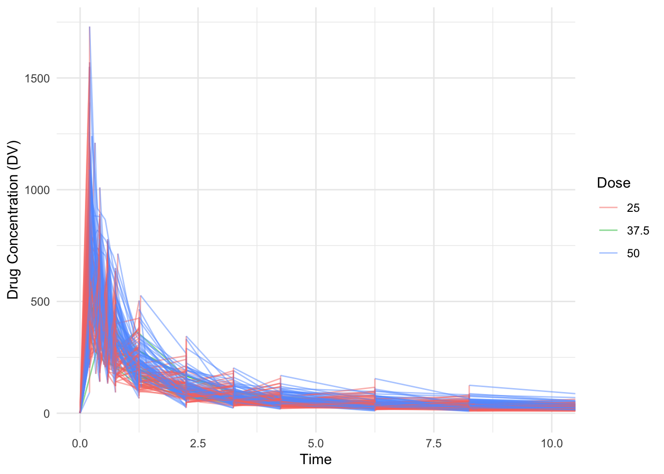
$ DV   <dbl> 0.00, 491.00, 605.00, 556.00, 310.00, 237.00, 147.00, 101.00, 72.…
$ LNDV <dbl> 0.000, 6.196, 6.405, 6.321, 5.737, 5.468, 4.990, 4.615, 4.282, 3.…
$ AMT  <dbl> 25, 0, 0, 0, 0, 0, 0, 0, 0, 0, 0, 0, 0, 0, 0, 0, 25, 0, 0, 0, 0, …
$ TIME <dbl> 0.000, 0.200, 0.250, 0.367, 0.533, 0.700, 1.200, 2.200, 3.200, 4.…
$ DOSE <dbl> 25, 25, 25, 25, 25, 25, 25, 25, 25, 25, 25, 25, 25, 25, 25, 25, 2…
$ OCC  <dbl> 1, 1, 1, 1, 1, 1, 1, 1, 1, 1, 1, 1, 1, 1, 1, 1, 1, 1, 1, 1, 1, 1,…
$ RATE <dbl> 75, 0, 0, 0, 0, 0, 0, 0, 0, 0, 0, 0, 0, 0, 0, 0, 150, 0, 0, 0, 0,…
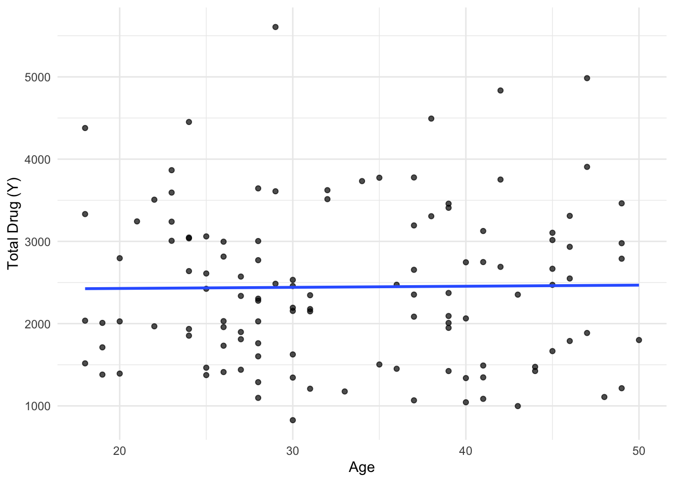
$ AGE  <dbl> 42, 42, 42, 42, 42, 42, 42, 42, 42, 42, 42, 42, 42, 42, 42, 42, 2…
$ SEX  <dbl> 1, 1, 1, 1, 1, 1, 1, 1, 1, 1, 1, 1, 1, 1, 1, 1, 1, 1, 1, 1, 1, 1,…
$ RACE <dbl> 2, 2, 2, 2, 2, 2, 2, 2, 2, 2, 2, 2, 2, 2, 2, 2, 2, 2, 2, 2, 2, 2,…
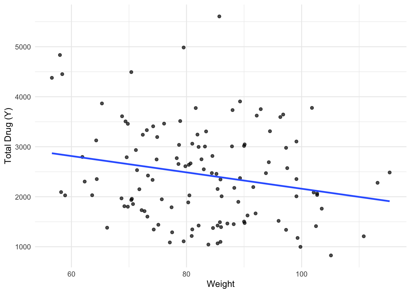
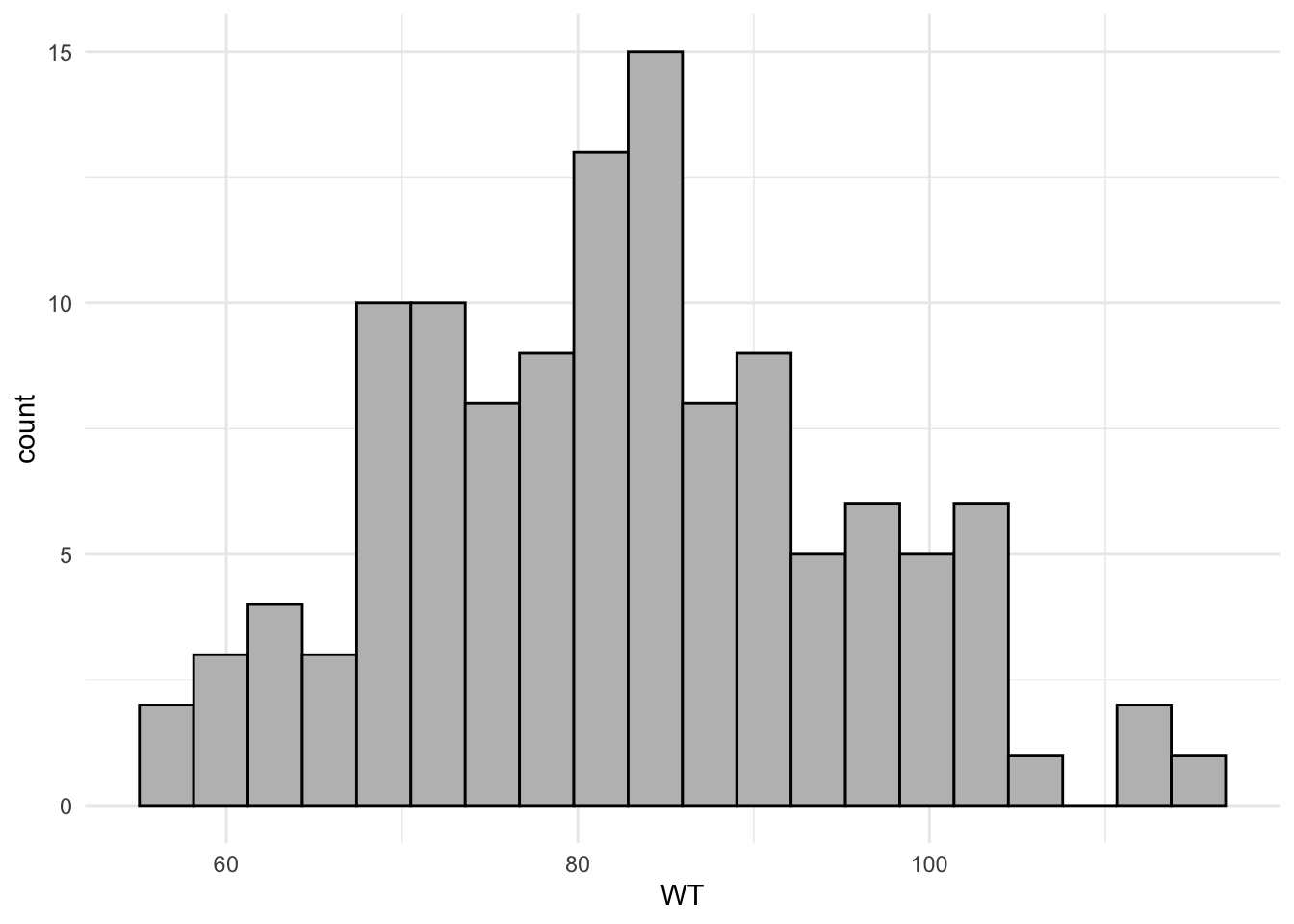
$ WT   <dbl> 94.3, 94.3, 94.3, 94.3, 94.3, 94.3, 94.3, 94.3, 94.3, 94.3, 94.3,…
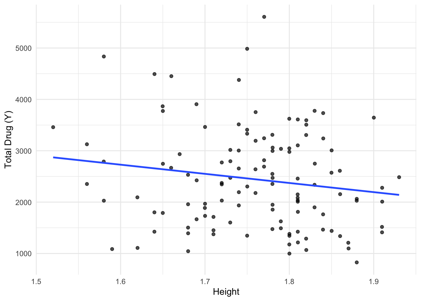
$ HT   <dbl> 1.769997, 1.769997, 1.769997, 1.769997, 1.769997, 1.769997, 1.769…

str(data)

spc_tbl_ [2,678 × 17] (S3: spec_tbl_df/tbl_df/tbl/data.frame)
 $ ID  : num [1:2678] 793 793 793 793 793 793 793 793 793 793 ...
 $ CMT : num [1:2678] 1 2 2 2 2 2 2 2 2 2 ...
 $ EVID: num [1:2678] 1 0 0 0 0 0 0 0 0 0 ...
 $ EVI2: num [1:2678] 1 0 0 0 0 0 0 0 0 0 ...
 $ MDV : num [1:2678] 1 0 0 0 0 0 0 0 0 0 ...
 $ DV  : num [1:2678] 0 491 605 556 310 237 147 101 72.4 52.6 ...
 $ LNDV: num [1:2678] 0 6.2 6.41 6.32 5.74 ...
 $ AMT : num [1:2678] 25 0 0 0 0 0 0 0 0 0 ...
 $ TIME: num [1:2678] 0 0.2 0.25 0.367 0.533 0.7 1.2 2.2 3.2 4.2 ...
 $ DOSE: num [1:2678] 25 25 25 25 25 25 25 25 25 25 ...
 $ OCC : num [1:2678] 1 1 1 1 1 1 1 1 1 1 ...
 $ RATE: num [1:2678] 75 0 0 0 0 0 0 0 0 0 ...
 $ AGE : num [1:2678] 42 42 42 42 42 42 42 42 42 42 ...
 $ SEX : num [1:2678] 1 1 1 1 1 1 1 1 1 1 ...
 $ RACE: num [1:2678] 2 2 2 2 2 2 2 2 2 2 ...
 $ WT  : num [1:2678] 94.3 94.3 94.3 94.3 94.3 94.3 94.3 94.3 94.3 94.3 ...
 $ HT  : num [1:2678] 1.77 1.77 1.77 1.77 1.77 ...
 - attr(*, "spec")=
  .. cols(
  ..   ID = col_double(),
  ..   CMT = col_double(),
  ..   EVID = col_double(),
  ..   EVI2 = col_double(),
  ..   MDV = col_double(),
  ..   DV = col_double(),
  ..   LNDV = col_double(),
  ..   AMT = col_double(),
  ..   TIME = col_double(),
  ..   DOSE = col_double(),
  ..   OCC = col_double(),
  ..   RATE = col_double(),
  ..   AGE = col_double(),
  ..   SEX = col_double(),
  ..   RACE = col_double(),
  ..   WT = col_double(),
  ..   HT = col_double()
  .. )
 - attr(*, "problems")=<externalptr> 

head(data)

# A tibble: 6 × 17
     ID   CMT  EVID  EVI2   MDV    DV  LNDV   AMT  TIME  DOSE   OCC  RATE   AGE
  <dbl> <dbl> <dbl> <dbl> <dbl> <dbl> <dbl> <dbl> <dbl> <dbl> <dbl> <dbl> <dbl>
1   793     1     1     1     1     0  0       25 0        25     1    75    42
2   793     2     0     0     0   491  6.20     0 0.2      25     1     0    42
3   793     2     0     0     0   605  6.40     0 0.25     25     1     0    42
4   793     2     0     0     0   556  6.32     0 0.367    25     1     0    42
5   793     2     0     0     0   310  5.74     0 0.533    25     1     0    42
6   793     2     0     0     0   237  5.47     0 0.7      25     1     0    42
# ℹ 4 more variables: SEX <dbl>, RACE <dbl>, WT <dbl>, HT <dbl>

Visualizing the data: Plot DV vs. Time for each individual (stratified by DOSE) The code below will result in drug concentration (DV) as a function of time, stratified by DOSE and using ID as a grouping factor. The plot shows a line for each individual, with DV on the y-axis and time on the x-axis. Stratified by dose (red - 25 ; green - 37.5 and blue - 50).

ggplot(data, aes(x = TIME, y = DV, group = ID, color = factor(DOSE))) +
  geom_line(alpha = 0.5) +
  labs(
    x = "Time",
    y = "Drug Concentration (DV)",
    color = "Dose"
  ) +
  theme_minimal() +
  coord_cartesian(xlim = c(0, 10))

In this graph is already possible to notice that drug concentration per time is higher for dose 50 compared to dose 25.

Remove observations with OCC = 2 Some individuals have multiple dosing occasions (OCC = 1 and OCC = 2). To simplify the analysis, we keep only OCC = 1.

data_occ1 <- data %>%
  filter(OCC == 1)

# Check that only OCC = 1 remains
table(data_occ1$OCC)

   1 
1665 

Compute total DV for each individual:

# Rows where TIME = 0 represent dosing events, not measurements. Remove these rows before computing the total drug concentration.
dv_sum <- data_occ1 %>%
  filter(TIME != 0) %>%      # remove dosing records
  group_by(ID) %>%           # group data by individual
  summarize(
    Y = sum(DV, na.rm = TRUE)   # sum of DV values per individual
  )

# Check the resulting dataset
dim(dv_sum)   # should be 120 x 2

[1] 120   2

head(dv_sum)

# A tibble: 6 × 2
     ID     Y
  <dbl> <dbl>
1   793 2691.
2   794 2639.
3   795 2150.
4   796 1789.
5   797 3126.
6   798 2337.

# Extract baseline observations (TIME = 0). These rows contain subject-level information such as dose, age, sex, race, weight, height, etc.
dose_data <- data_occ1 %>%
  filter(TIME == 0)

# Verify dimensions
dim(dose_data)   # should be 120 x 17

[1] 120  17

# Combine outcome variable with subject covariates
# Join the DV summary (Y) with the baseline subject data using ID
combined_data <- dv_sum %>%
  left_join(dose_data, by = "ID")

# Check dimensions of the merged dataset
dim(combined_data)   # should be 120 x 18

[1] 120  18

# Final cleaning and variable selection. Convert categorical variables to factors
# Keep only variables required for the analysis

final_data <- combined_data %>%
  mutate(
    SEX = factor(SEX),
    RACE = factor(RACE)
  ) %>%
  select(
    Y, DOSE, AGE, SEX, RACE, WT, HT
  )

# Inspect the final dataset
glimpse(final_data)

Rows: 120
Columns: 7
$ Y    <dbl> 2690.52, 2638.81, 2149.61, 1788.89, 3126.37, 2336.89, 3007.20, 27…
$ DOSE <dbl> 25.0, 25.0, 25.0, 25.0, 25.0, 25.0, 25.0, 25.0, 25.0, 25.0, 25.0,…
$ AGE  <dbl> 42, 24, 31, 46, 41, 27, 23, 20, 23, 28, 46, 22, 43, 50, 19, 26, 3…
$ SEX  <fct> 1, 1, 1, 2, 2, 1, 1, 1, 1, 1, 1, 1, 2, 2, 1, 1, 1, 1, 1, 1, 1, 1,…
$ RACE <fct> 2, 2, 1, 1, 2, 2, 1, 88, 2, 1, 1, 1, 1, 1, 2, 2, 1, 1, 1, 1, 1, 1…
$ WT   <dbl> 94.3, 80.4, 71.8, 77.4, 64.3, 74.1, 87.9, 61.9, 65.3, 103.5, 83.0…
$ HT   <dbl> 1.769997, 1.759850, 1.809847, 1.649993, 1.560052, 1.829862, 1.850…

summary(final_data)

       Y               DOSE            AGE        SEX     RACE   
 Min.   : 826.4   Min.   :25.00   Min.   :18.00   1:104   1 :74  
 1st Qu.:1700.5   1st Qu.:25.00   1st Qu.:26.00   2: 16   2 :36  
 Median :2349.1   Median :37.50   Median :31.00           7 : 2  
 Mean   :2445.4   Mean   :36.46   Mean   :33.00           88: 8  
 3rd Qu.:3050.2   3rd Qu.:50.00   3rd Qu.:40.25                  
 Max.   :5606.6   Max.   :50.00   Max.   :50.00                  
       WT               HT       
 Min.   : 56.60   Min.   :1.520  
 1st Qu.: 73.17   1st Qu.:1.700  
 Median : 82.10   Median :1.770  
 Mean   : 82.55   Mean   :1.759  
 3rd Qu.: 90.10   3rd Qu.:1.813  
 Max.   :115.30   Max.   :1.930  

# Confirm final dataset size
dim(final_data)  

[1] 120   7

EDA on the cleaned dataset (final_data)

The goal here is to explore relationships, distributions, and summaries so you understand the data before modeling.

# Summary statistics for all variables
summary(final_data)

       Y               DOSE            AGE        SEX     RACE   
 Min.   : 826.4   Min.   :25.00   Min.   :18.00   1:104   1 :74  
 1st Qu.:1700.5   1st Qu.:25.00   1st Qu.:26.00   2: 16   2 :36  
 Median :2349.1   Median :37.50   Median :31.00           7 : 2  
 Mean   :2445.4   Mean   :36.46   Mean   :33.00           88: 8  
 3rd Qu.:3050.2   3rd Qu.:50.00   3rd Qu.:40.25                  
 Max.   :5606.6   Max.   :50.00   Max.   :50.00                  
       WT               HT       
 Min.   : 56.60   Min.   :1.520  
 1st Qu.: 73.17   1st Qu.:1.700  
 Median : 82.10   Median :1.770  
 Mean   : 82.55   Mean   :1.759  
 3rd Qu.: 90.10   3rd Qu.:1.813  
 Max.   :115.30   Max.   :1.930  

#Compute summary statistics by dose group:
final_data %>%
  group_by(DOSE) %>%
  summarize(
    mean_Y = mean(Y),
    sd_Y = sd(Y),
    min_Y = min(Y),
    max_Y = max(Y),
    n = n()
  )

# A tibble: 3 × 6
   DOSE mean_Y  sd_Y min_Y max_Y     n
  <dbl>  <dbl> <dbl> <dbl> <dbl> <int>
1  25    1783.  601.  826. 3866.    59
2  37.5  2464.  488. 1801. 3463.    12
3  50    3239.  787. 1949. 5607.    49

#Counts for categorical variables:
table(final_data$SEX)

  1   2 
104  16 

table(final_data$RACE)

 1  2  7 88 
74 36  2  8 

table(final_data$DOSE)

  25 37.5   50 
  59   12   49 

Y vs Age

ggplot(final_data, aes(x = AGE, y = Y)) +
  geom_point(alpha = 0.7) +
  geom_smooth(method = "lm", se = FALSE) +
  labs(x = "Age", y = "Total Drug (Y)") +
  theme_minimal()

`geom_smooth()` using formula = 'y ~ x'

Y vs Weight

ggplot(final_data, aes(x = WT, y = Y)) +
  geom_point(alpha = 0.7) +
  geom_smooth(method = "lm", se = FALSE) +
  labs(x = "Weight", y = "Total Drug (Y)") +
  theme_minimal()

`geom_smooth()` using formula = 'y ~ x'

Y vs Height

ggplot(final_data, aes(x = HT, y = Y)) +
  geom_point(alpha = 0.7) +
  geom_smooth(method = "lm", se = FALSE) +
  labs(x = "Height", y = "Total Drug (Y)") +
  theme_minimal()

`geom_smooth()` using formula = 'y ~ x'

Boxplots:

Y vs Dose

ggplot(final_data, aes(x = factor(DOSE), y = Y)) +
  geom_boxplot() +
  labs(x = "Dose", y = "Total Drug (Y)") +
  theme_minimal()

Y vs Sex

ggplot(final_data, aes(x = SEX, y = Y)) +
  geom_boxplot() +
  labs(x = "Sex", y = "Total Drug (Y)") +
  theme_minimal()

Y vs Race

ggplot(final_data, aes(x = RACE, y = Y)) +
  geom_boxplot() +
  labs(x = "Race", y = "Total Drug (Y)") +
  theme_minimal()

For both the Race and Sex categorical variables, there appear to be some differences in total drug exposure (Y) across the different categories. However, the dataset does not specify what the categories represent. For example, it is not clear whether the values 0 or 1 in the Sex variable correspond to male or female, which makes the interpretation of these differences more difficult.

Distribution plots for numeric variables:

#Distribution of Age: 
ggplot(final_data, aes(x = AGE)) +
  geom_histogram(bins = 20, fill = "gray", color = "black") +
  theme_minimal()

#Distribution of Weight: 
ggplot(final_data, aes(x = WT)) +
  geom_histogram(bins = 20, fill = "gray", color = "black") +
  theme_minimal()

Correlation Matrix to detect what variables are related to each other:

# Select numeric variables
numeric_data <- final_data %>%
  select(Y, DOSE, AGE, WT, HT)

# Correlation matrix
cor(numeric_data)

               Y       DOSE         AGE         WT          HT
Y     1.00000000 0.71808396  0.01256372 -0.2128719 -0.15832972
DOSE  0.71808396 1.00000000  0.07201600  0.1012319  0.01877994
AGE   0.01256372 0.07201600  1.00000000  0.1196740 -0.35185806
WT   -0.21287194 0.10123185  0.11967399  1.0000000  0.59975050
HT   -0.15832972 0.01877994 -0.35185806  0.5997505  1.00000000

The strongest relationship is between dose (DOSE) and total drug exposure (Y), with a correlation of about 0.72, which indicates a strong positive association. This means that higher doses generally lead to higher overall drug concentrations, which is what we would expect. The relationship between age and Y is very close to zero, suggesting that age does not have much influence on the total drug exposure in this dataset. Weight and height show weak negative correlations with Y, meaning that larger individuals may have slightly lower drug concentrations, but the relationship is not very strong. As expected, weight and height are moderately correlated, since taller individuals tend to weigh more. Overall, the results suggest that dose is the main factor related to differences in total drug exposure, while the other variables appear to have much smaller effects.

Model Fitting:

I used the tidymodels framework to fit simple predictive models. We first fit linear models where the outcome is the continuous variable Y, and then logistic models where the outcome is the categorical variable SEX.

library(tidymodels)

── Attaching packages ────────────────────────────────────── tidymodels 1.4.1 ──

✔ broom        1.0.12     ✔ rsample      1.3.2 
✔ dials        1.4.2      ✔ tailor       0.1.0 
✔ infer        1.1.0      ✔ tune         2.0.1 
✔ modeldata    1.5.1      ✔ workflows    1.3.0 
✔ parsnip      1.4.1      ✔ workflowsets 1.1.1 
✔ recipes      1.3.1      ✔ yardstick    1.3.2 

Warning: package 'broom' was built under R version 4.4.3

Warning: package 'infer' was built under R version 4.4.3

Warning: package 'parsnip' was built under R version 4.4.3

Warning: package 'rsample' was built under R version 4.4.3

── Conflicts ───────────────────────────────────────── tidymodels_conflicts() ──
✖ scales::discard() masks purrr::discard()
✖ dplyr::filter()   masks stats::filter()
✖ recipes::fixed()  masks stringr::fixed()
✖ dplyr::lag()      masks stats::lag()
✖ yardstick::spec() masks readr::spec()
✖ recipes::step()   masks stats::step()

#Split the data so that we can evaluate model performance on unseen data.
set.seed(123)

data_split <- initial_split(final_data, prop = 0.8)

train_data <- training(data_split)
test_data  <- testing(data_split)

Testing models:

Model 1: Y predicted by DOSE

#define model
lm_model_dose <- linear_reg() %>%
  set_engine("lm")
#fit the model
lm_fit_dose <- lm_model_dose %>%
  fit(Y ~ DOSE, data = train_data)
#predict:
pred_dose <- predict(lm_fit_dose, test_data) %>%
  bind_cols(test_data)

metrics(pred_dose, truth = Y, estimate = .pred)

# A tibble: 3 × 3
  .metric .estimator .estimate
  <chr>   <chr>          <dbl>
1 rmse    standard     483.   
2 rsq     standard       0.687
3 mae     standard     359.   

The model explains about 69% of the variability in Y, as shown by the R-squared value of 0.687. This indicates a relatively strong relationship between dose and total drug exposure, which is expected since higher doses should generally produce higher drug concentrations.

Model 2: Y predicted by all predictors

lm_fit_all <- lm_model_dose %>%
  fit(Y ~ DOSE + AGE + SEX + RACE + WT + HT, data = train_data)

pred_all <- predict(lm_fit_all, test_data) %>%
  bind_cols(test_data)

metrics(pred_all, truth = Y, estimate = .pred)

# A tibble: 3 × 3
  .metric .estimator .estimate
  <chr>   <chr>          <dbl>
1 rmse    standard     494.   
2 rsq     standard       0.662
3 mae     standard     374.   

The linear regression model including all predictors (DOSE, AGE, SEX, RACE, WT, and HT) does not improve the model performance compared to the simpler model using only DOSE. The R² value slightly decreases and the RMSE increases, indicating that the model with additional predictors performs slightly worse. This suggests that dose is the main factor explaining variation in total drug exposure (Y), while the other variables do not contribute much additional predictive power in this dataset.

Model 3: SEX predicted by DOSE

#Define regression model

log_model_dose <- logistic_reg() %>%
  set_engine("glm")

#Fit model
log_fit_dose <- log_model_dose %>%
  fit(SEX ~ DOSE, data = train_data)

#Predict:
pred_sex_dose <- predict(log_fit_dose, test_data, type = "prob") %>%
  bind_cols(
    predict(log_fit_dose, test_data),
    test_data
  )

#evaluate accuracy and ROC-AUC:
accuracy(pred_sex_dose, truth = SEX, estimate = .pred_class)

# A tibble: 1 × 3
  .metric  .estimator .estimate
  <chr>    <chr>          <dbl>
1 accuracy binary         0.917

roc_auc(pred_sex_dose, truth = SEX, .pred_1)

# A tibble: 1 × 3
  .metric .estimator .estimate
  <chr>   <chr>          <dbl>
1 roc_auc binary           0.5

The logistic regression model predicting SEX from DOSE shows an accuracy of about 0.92, meaning that most observations were classified correctly. However, the ROC-AUC value is 0.5, which indicates that the model has no real predictive ability and performs similarly to random guessing. The high accuracy is likely due to an imbalance in the SEX categories, where one category appears more frequently than the other. Overall, this result makes sense scientifically, since drug dose should not be expected to predict a person’s sex.

Model 4: SEX predicted by all predictors

log_fit_all <- log_model_dose %>%
  fit(SEX ~ DOSE + AGE + RACE + WT + HT + Y, data = train_data)

Warning: glm.fit: fitted probabilities numerically 0 or 1 occurred

pred_sex_all <- predict(log_fit_all, test_data, type = "prob") %>%
  bind_cols(
    predict(log_fit_all, test_data),
    test_data
  )

accuracy(pred_sex_all, truth = SEX, estimate = .pred_class)

# A tibble: 1 × 3
  .metric  .estimator .estimate
  <chr>    <chr>          <dbl>
1 accuracy binary         0.875

roc_auc(pred_sex_all, truth = SEX, .pred_1)

# A tibble: 1 × 3
  .metric .estimator .estimate
  <chr>   <chr>          <dbl>
1 roc_auc binary         0.955

The logistic regression model predicting SEX using all predictors shows an accuracy of about 0.88 and a ROC-AUC of 0.96, suggesting that the model can distinguish between the two categories fairly well. However, in my view this result should be interpreted with caution, from a biology point of view drug dose or exposure should not determine sex. Maybe this is a problem with this small dataset where weight or others variables can be misrepresented among the sex categories.

Extra: k-Nearest Neighbors (kNN):

kNN is a non-parametric machine learning model used for (a) Regression → predicting a numeric outcome or (b) Classification → predicting categories. Instead of fitting an equation like linear regression, kNN works by looking at similar observations in the dataset.

Code for kNN regression (tidymodels)

library(kknn)

# Define kNN regression model
knn_model <- nearest_neighbor(neighbors = 5) %>%
  set_engine("kknn") %>%
  set_mode("regression")

# Fit the model
knn_fit <- knn_model %>%
  fit(Y ~ DOSE + AGE + WT + HT, data = train_data)

# Make predictions
knn_pred <- predict(knn_fit, test_data) %>%
  bind_cols(test_data)

# Evaluate performance
metrics(knn_pred, truth = Y, estimate = .pred)

# A tibble: 3 × 3
  .metric .estimator .estimate
  <chr>   <chr>          <dbl>
1 rmse    standard     645.   
2 rsq     standard       0.560
3 mae     standard     545.   

A k-nearest neighbors regression model was also fitted to predict total drug exposure (Y). The performance of the kNN model was worse than the linear regression models, with a higher RMSE and a lower R² value. This suggests that the relationship between dose and total drug exposure is relatively simple and can be captured well by both linear model and k-nearest model. In this case, the kNN approach does not improve predictive performance.

Module 10: Model Improvement

Model performance assessment 1: Prepare data by removing RACE variable and split dataset into 75/25

#Step 1: remove RACE variable:
final_data2 <- final_data %>%
  select(-RACE)

#Set seed for random variability
rngseed = 1234
set.seed(rngseed)

#75/25 split
data_split <- initial_split(final_data2, prop = 0.75)
train_data <- training(data_split)
test_data <- testing(data_split)

Now, define model:

# Linear regression model
lm_model <- linear_reg() %>%
  set_engine("lm")

Fit the two models using the training data only:

Model 1: DOSE only

lm_fit_dose <- lm_model %>%
  fit(Y ~ DOSE, data = train_data)

Model 2: all predictors

lm_fit_all <- lm_model %>%
  fit(Y ~ DOSE + AGE + SEX + WT + HT, data = train_data)

Predictions on training data

# Model 1 predictions
pred_dose_train <- predict(lm_fit_dose, train_data) %>%
  bind_cols(train_data)

# Model 2 predictions
pred_all_train <- predict(lm_fit_all, train_data) %>%
  bind_cols(train_data)

Compute RMSE for both models:

rmse_dose <- rmse(pred_dose_train, truth = Y, estimate = .pred)
rmse_all  <- rmse(pred_all_train, truth = Y, estimate = .pred)

rmse_dose

# A tibble: 1 × 3
  .metric .estimator .estimate
  <chr>   <chr>          <dbl>
1 rmse    standard        703.

rmse_all

# A tibble: 1 × 3
  .metric .estimator .estimate
  <chr>   <chr>          <dbl>
1 rmse    standard        627.

Null model:

# Compute mean of Y in training data
mean_Y <- mean(train_data$Y)

# Create predictions = mean
null_pred <- train_data %>%
  mutate(.pred = mean_Y)

# Compute RMSE
rmse_null <- rmse(null_pred, truth = Y, estimate = .pred)

rmse_null

# A tibble: 1 × 3
  .metric .estimator .estimate
  <chr>   <chr>          <dbl>
1 rmse    standard        948.

The null model, which just predicts the average value of Y for everyone, has the highest RMSE (~948), so it performs the worst. That makes sense since it doesn’t use any information from the predictors. Model 1, using only DOSE, brings the RMSE down quite a bit (~703), which shows that dose alone explains a large part of the variation in total drug exposure. Model 2, which includes all predictors (DOSE, AGE, SEX, WT, HT), has the lowest RMSE (~627), so it performs the best out of the three.

Overall, this suggests that DOSE is the main factor driving drug exposure, but the other variables add a bit of extra predictive power.

Model performance assessment 2:

Set seed again and create cv_folds:

set.seed(1234)

cv_folds <- vfold_cv(train_data, v = 10)

Fit models using cross-validation:

Model 1: DOSE only:

cv_fit_dose <- lm_model %>%
  fit_resamples(
    Y ~ DOSE,
    resamples = cv_folds,
    metrics = metric_set(rmse)
  )

Model 2 (all predictors):

cv_fit_all <- lm_model %>%
  fit_resamples(
    Y ~ DOSE + AGE + SEX + WT + HT,
    resamples = cv_folds,
    metrics = metric_set(rmse)
  )

Extract RMSE results:

collect_metrics(cv_fit_dose)

# A tibble: 1 × 6
  .metric .estimator  mean     n std_err .config        
  <chr>   <chr>      <dbl> <int>   <dbl> <chr>          
1 rmse    standard    691.    10    67.5 pre0_mod0_post0

collect_metrics(cv_fit_all)

# A tibble: 1 × 6
  .metric .estimator  mean     n std_err .config        
  <chr>   <chr>      <dbl> <int>   <dbl> <chr>          
1 rmse    standard    646.    10    64.8 pre0_mod0_post0

Using 10-fold cross-validation, the RMSE values are slightly different from those obtained on the training data. Model 1 (DOSE only) has an RMSE of about 691, while Model 2 (all predictors) has an RMSE of about 646.

•   Model 1 from training RMSE = 703 → 691 entire dataset
•   Model 2 from training RMSE = 627 → 646 entire dataset

This section is added by Anissa Waller Del Valle

# null model predictions
mean_Y <- mean(train_data$Y)
pred_null_train <- train_data %>%
  mutate(.pred = mean_Y,
         model = "Null")

# model 1 predictions (DOSE)
pred_dose_train <- predict(lm_fit_dose, train_data) %>%
  bind_cols(train_data) %>%
  mutate(model = "Dose")

# model 2 predictions (all predictors)
pred_all_train <- predict(lm_fit_all, train_data) %>%
  bind_cols(train_data) %>%
  mutate(model = "All")

# combine all predictions
pred_combined <- bind_rows(
  pred_null_train,
  pred_dose_train,
  pred_all_train
)

# plot observed vs predicted
ggplot(pred_combined, aes(x = Y, y = .pred, color = model)) +
  geom_point(alpha = 0.6) +
  geom_abline(slope = 1, intercept = 0) +
  coord_cartesian(xlim = c(0, 5000), ylim = c(0, 5000)) +
  labs(x = "Observed", y = "Predicted") +
  theme_minimal()

The null model shows a flat horizontal line. This is expected, as it predicts the same mean value of Y for all observations. The dose only model shows three horizontal bands, which happens because dose only takes three values. The model with all predictors performs the best, with points closer to the diagnol line. There is some scatter (at higher observed values, seems underpredicted), suggesting that the model is missing some patterns in the data.

# Residuals vs predicted (model 2)

pred_all_train <- pred_all_train %>%
  mutate(residual = .pred - Y)

ggplot(pred_all_train, aes(x = .pred, y = residual)) +
  geom_point(alpha = 0.6) +
  geom_hline(yintercept = 0) +
  coord_cartesian(ylim = c(-2500, 2500)) +
  labs(x = "Predicted", y = "Residuals") +
  theme_minimal()

There is a lot of scatter. The spread is not even and has a large range. We are seeing more negative residuals at higher predicted values, suggesting that the model is underpredicting for larger Y values, consistent with prior findings. There may be missing patterns or variables.

# Bootstrap for model 2

library(rsample)

set.seed(1234)

# create bootstraps
dat_bs <- bootstraps(train_data, times = 100)

# store predictions
pred_bs <- matrix(NA, nrow = 100, ncol = nrow(train_data))

for(i in 1:100){
  
  dat_sample <- rsample::analysis(dat_bs$splits[[i]])
  
  fit_bs <- lm_model %>%
    fit(Y ~ DOSE + AGE + SEX + WT + HT, data = dat_sample)
  
  pred_bs[i, ] <- predict(fit_bs, train_data)$.pred
}

# compute median and CI
preds <- pred_bs |>
  apply(2, quantile, c(0.055, 0.5, 0.945)) |>
  t()

preds_df <- as.data.frame(preds)

# original predictions
orig_pred <- predict(lm_fit_all, train_data) %>%
  bind_cols(train_data)

# combine
plot_data <- orig_pred %>%
  mutate(
    median = preds_df$`50%`,
    lower = preds_df$`5.5%`,
    upper = preds_df$`94.5%`
  )

# plot
ggplot(plot_data, aes(x = Y)) +
  geom_point(aes(y = .pred), color = "black", alpha = 0.6) +
  geom_point(aes(y = median), color = "blue", alpha = 0.6) +
  geom_point(aes(y = lower), color = "red", alpha = 0.4) +
  geom_point(aes(y = upper), color = "red", alpha = 0.4) +
  geom_abline(slope = 1, intercept = 0) +
  coord_cartesian(xlim = c(0, 5000), ylim = c(0, 5000)) +
  labs(x = "Observed", y = "Predicted") +
  theme_minimal()

The data points follow a fairly diagnol trend, confirming that this model captures the overall relationship. However, there is a lot of spread (especially at higher observed values), indicating uncertainty. Like before, this suggests that the model is less reliable for larger Y values.

The model with all predictors performs better than the simpler models, although there is still uncertainty. The consistent higher under prediction at higher values and wide bootstrap variables indicate that the model is either TOO simple, even with the addition of all variables, or that there is important information missing.

This section was written again by Aylla von Ermland:

Predict on the test data: Using my already fitted model (lm_fit_all) and generate predictions for the test set:

# model 2 predictions on test data
pred_all_test <- predict(lm_fit_all, test_data) %>%
  bind_cols(test_data) %>%
  mutate(
    model = "All",
    dataset = "Test"
  )

#label training predictions:
pred_all_train <- pred_all_train %>%
  mutate(dataset = "Train")

#Combine train + test predictions:
pred_final <- bind_rows(
  pred_all_train,
  pred_all_test
)

Plot observed vs. predicted:

ggplot(pred_final, aes(x = Y, y = .pred, color = dataset)) +
  geom_point(alpha = 0.6) +
  geom_abline(slope = 1, intercept = 0) +
  coord_cartesian(xlim = c(0, 5000), ylim = c(0, 5000)) +
  labs(
    x = "Observed",
    y = "Predicted",
    color = "Dataset"
  ) +
  theme_minimal()

Overall model assessment:

Overall, all models do better than the null model, which is good; the null just predicts the mean and clearly doesn’t capture any real pattern. The Model 1 (dose only) is a small improvement over the null. It makes sense that dose has some effect, but the predictions fall into just a few bands, which is pretty limiting, I wouldn’t consider this model useful for real world prediction. The Model 2 (all predictors) definitely improves things. The RMSE is lower, and the predicted vs observed plot shows points closer to the diagonal. The test data also lines up well with the training data, which suggests the model perform reasonably well and isn’t bad overfit, I would use for “real” world purpose.